Consistency training II: How does it work?
Corresponding code in this Colab
In consistency training we’re not mapping from inputs to outputs like in supervised learning. The only thing we’re telling the model is to respond in the same way to different perturbations of the same input image. We’re not telling the model how to behave at all, we’re simply telling it to behave consistently.
How on Earth does that create useful features? We’ll explain with another example.
You’ve been given the task of creating a banana vs. plum classifier. Just those two classes. You only have unlabeled data to start with, but you can expect to get a small amount of labels soon.
You don’t know which class is which, but can you guess where the decision boundary will be in the dataset below?
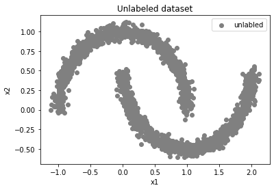
Good guess. We know intuitively that decision boundaries shouldn’t cut through high-density clusters of data. They should slide into place only in the low-density regions between clusters. This is called the “cluster assumption”—it’s the core motivation behind all of consistency training. One upshot to the cluster assumption is that we can make educated guesses on where decision boundaries should be without any labels at all.
Let’s add some labels.
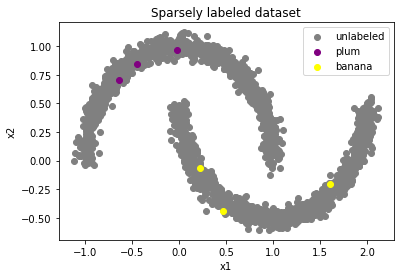
As humans, this should be enough for us to get 100% accuracy on the task. We already knew where the dividing line was, now we can guess with confidence which class is which. Humans are easily able to propagate the label from a single example throughout the entire cluster. Supervised learning models on the other hand…
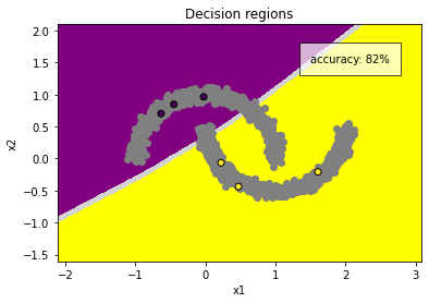
Not very good. It’s ignoring all the unlabeled data points. It’s not a problem with model capacity, we’re using a three-layer MLP that could easily fit half-moons if we had more labels.
Maybe we can squeeze out a bit more accuracy with data augmentation? Let’s randomly jitter our input properties x1 and x2. This is a lower-dimension analogue of what we do in computer vision with the standard set of augmentations (crop, rotation, color jitter, etc.).
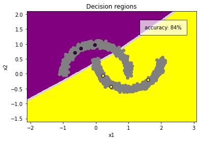
Not any better. We’re only able to propagate our labels throughout a small zone directly around each respective point. Enforcing invariance on only six data points isn’t enough to push our decision boundaries away any further than they already are.
Like we said in the intro, if we’re willing to enforce an invariance constraint on our labeled records, we should be willing (eager!) to enforce it across all our records. Let’s zoom in on a few unlabelled points and see what that looks like under the microscope.
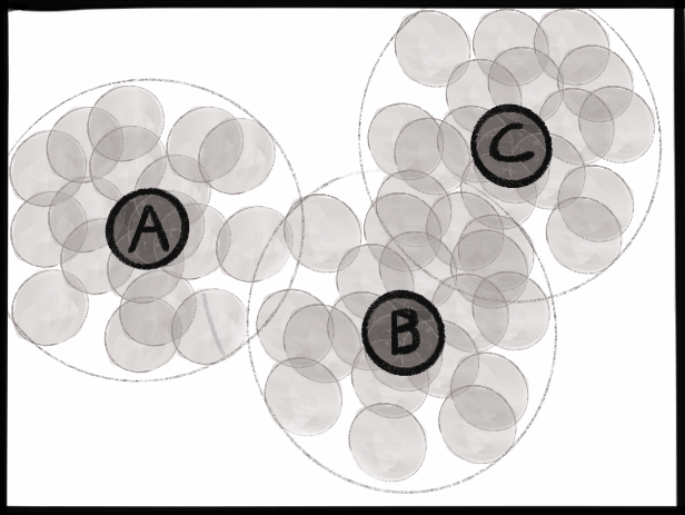 The original three points ‘A’, ‘B’ and ‘C’ are colored dark. Each seed point is surrounded by a cloud of different “views” of that point, i.e. data augmentations, effectively filling out the dataset. The model is agnostic to any differentiation within each cloud. Each cloud is outlined for visual clarity.
We’re telling the model that all points within each zone are identical to all the other points within the same zone. But the zones overlap! If all the points in zone ‘A’ are identical, and all the points in zone ‘B’ are identical, and all the points in zone ‘C’ are identical, then ALL the points in the entire macro zone are identical. We’ve collapsed all differentiation within that blob. Our specific choice of data augmentation is critical—the boundary of the “zone of invariance” is delineated exactly by our amount of augmentation.
When we do this across the whole dataset—if we’ve chosen our data augmentations well—then all of the points within each halfmoon cluster will be linked together. We’ll be left with two contiguous, fortified zones of invariance, neither of which will admit a decision boundary.
Now when we drop in our labeled data points their labels spread like wildfire to all the unlabeled points in each of their respective clusters, exactly what we did mentally when we first saw the labels.
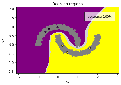
100% accuracy with only six labeled examples! Our consistency training told the model that the decision boundary can’t cut through either of the clusters, and the labelled examples told the model which side of the boundary should belong to which class. With those two constraints, the model had no choice but to draw the decision boundary where we wanted it.
Appendix
Let’s see what’s happening in feature-space when we do only consistency training, no labels. We’ll use the NCE loss, which not only pulls views of the same record together but also pushes them apart from other records. We talked about this loss in more detail in An engineer’s guide to the literature.
As you can see below, consistency training separates our clusters even without using any labels. The points in each contiguous zone are pulled together while simultaneously being pushed away from any unlinked bodies.
Consistency training pulls ‘positives’ together and pushes ‘negatives’ apart in feature-space. Points are colored by class for visual clarity, but the model doesn’t see that—this is entirely unsupervised.
We’ve chosen the “golidlocks” amount of augmentation for this example—too much data augmentation and both halfmoons would have collapsed into a single blob, too little and nothing will agglomerate at all.
Next post: Consistency training III: An engineer’s guide to the literature
Previous post: Consistency training I: Intro